Learning curves and cross-validation

Two very useful concepts!

Learning curves and cross-validation are integral things to incorporate when training your models. Learning curves help clue you in on how much labeled data you need and crucially helps inform you about whether your model is overfitting or underfitting. Cross-validation allows you to monitor and helps to reduce bias and variance, and is a necessary inclusion in your aforementioned learning curves in order to spot overfitting and underfitting. I’ll start with talking about cross-validation.

Cross-validation

Cross-validation draws from a validation set. I mentioned it briefly in the first part of this series of ML posts. A validation set is a test set that is used during training, and typically takes the same percentage of the labeled data as the test set. Cross-validation aims to continually assess a model’s ability to generalize as it’s being trained. The most common form of cross-validation is the non-exhaustive \(k\)-fold cross-validation.

\(k\)-fold cross-validation

In \(k\)-fold cross-validation, a fold is the size of the training data to be partitioned into \(k\) equally sized subsets. Of the \(k\) folds, \(k-1\) folds are used for training and one fold is reserved as a test set. From this partition, a model is trained on the training part and an accuracy score is computed on the test part of each fold. The scores from each of the folds are averaged and used as an evaluation metric. An image of this process, created by Wikipedia user Gufosawa, can be found below:

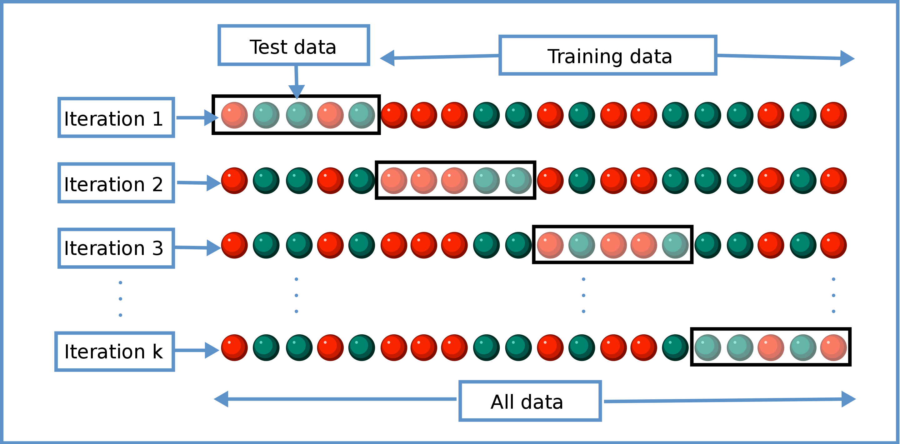
As you can see, the test data is a sliding window that glides over the whole dataset per epoch, such that every datapoint is used once and only once as test data.

From my article on the basics of ML I talk about there being some ideal function \(\hat f\) that we wish to approximate. One can imagine there being some set of approximating functions \(\{f_i\}^n\) with varying effectiveness. The best approximator \(\bar f\) in that set will have the lowest total variance and bias compared to its fellow members in the set. Cross-validation is good because it serves as a very useful evaluation metric to assist in finding \(\bar f\).

Rewriting the loss function

If you take a look at the loss function I made in my previously mentioned article, you’ll note that it’s actually just an average of the squared difference between the true and predicted values of a dataset:

\[\mathcal{L} = \sum_{i=1}^n \left(y_i - f(x_i)\right)^2\]

which is often called the residual sum of squares, or the mean squared error, or MSE. The mean is called an expected value, and can actually be written more simply as this:

\[\mathcal{L} = \sum_{i=1}^n \left(y_i - f(x_i)\right)^2 = \mathbb{E}\left[\left(y_i - f(x_i)\right)^2\right]\]

and there’s actually a way of rewriting this equation:

\[\mathbb E\left[\left(y_i - f(x_i)\right)^2\right] = \mathbb E\left[y_i - f(x_i)\right]^2 +\mathbb E\left[\left(f(x_i) - \mathbb E\left[f(x_i)\right] \right)^2\right]\]

Of that new expression on the right-hand side, the first term is called the square of the expected bias, and the second term is called the variance of the estimator \(f\).

It’s clear to see that to minimize loss, you ideally need to minimize bias and variance together.

Bias and Variance

As you might be able to tell by looking at the term above and noting that it’s referring to the squared bias, bias is the average amount your estimator’s prediction \(f(x_i)\) is off from the true value \(y_i\). On the other hand, variance is the average amount your predicted values are displaced from your average predicted value.

This may seem a bit vague, but bias and variance are antithetical to accuracy and precision respectively, which is one of the first things most physics undergraduates learn about when doing experiments. Both accuracy, bias, variance and precision can be really well described with a dartboard like in the image below (Dusen et al).

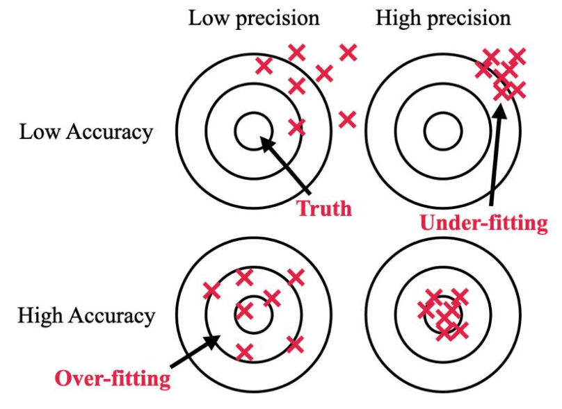
Bias, like accuracy, is concerned with, on average, how close darts (predicted values) are to the bullseye (true values) in that if a dart hits the bullseye, then one of your predicted values was equal to its true value, while variance, like precision, is concerned with how close darts (predicted values) are to eachother. Just like the image describes, an under-fitted model (equating to high bias but low variance) leads to “low accuracy, but high precision” and an overfitted model (equating to high variance and low bias) “leads to low precision but high accuracy” (Dusen et al).

The two terms also tend to have a less mathematic but more qualitative definition that is also often more useful: bias is a systematic error in data due to oversimplistic learning, and variance is an error associated with sensitivity to perturbations in the training set, such as noise.

As an estimator becomes more complex, it’ll start to look like it’s “connecting the dots”, which reduces bias as predicted values will on average be closer to target values. However, the nature of this more all-over-the-place estimator will have a higher average distance from the average predicted value, thus having a higher variance. Lowering one tends to raise the other. This highlights something called the bias-variance tradeoff, which is one of the foremost problems with generalizing past a training set.

Cross-validation is really helpful in grappling with this problem.

Why is cross-validation a good idea?

The design of the \(k\)-fold cross-validation is able to flag for bias because by changing the test set per fold it’s continuously testing the model on new data (\(k\) times per epoch rather than once per epoch, which is done in a standard split), instead of optimizing on the same test set each epoch, and by performing multiple rounds of cross-validation variance is monitored by measuring the model’s predictive performance throughout the rounds, so that we can use it as an early stopping monitor if overfitting starts to occur. Bias can be inherent to your dataset, as biased datasets are a common headache among data scientists, but CV can at the very least reduce what bias it can by using all of the data for training and lowering variance by varying the test sets used to average out any perturbations, preventing any unhelpful updates to model parameters.

Cross-validation scores are a great way to monitor how your model is training, especially using learning curves.

Learning curves

Learning curves are plots of the scores of a model’s training score and cross-validation as training examples increase. It can help indicate whether your model suffers from a bias problem or a variance problem more, and when your model may benefit from more data. An example of which is shown below, provided by scikit-learn.

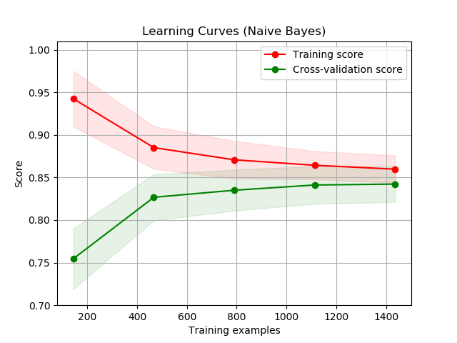
The training score is typically something like the MSE of points in the training set, while the cross-validation score concerns the MSE of points in the validation set. The score you see is the averaged score across all \(k\) folds for some given number of points. What you see below is pretty typical of a well-trained model. As the number of training examples increase, the two scores will tend to converge to some irreducible bias as both sets will have an adequate sample size to improve as far as it possibly can. The cross-validation getting better with more data makes sense, as you’d hope that as the model is introduced to more examples its ability to generalize on unseen data improves, and the training score decreases as the model is getting worse at overfitting.

Can you tell what the training curves would look like for overfit or underfit models? For high bias models, the training curve and validation curves would both likely be high (as this is a loss curve). You’d be able to tell that the model has high variance if the gap between curves was large, as an overfitted model will perform well on the training data and poorly on the validation data, and this can often be remedied by adding more data if it looks like the two lines are converging. For example, if you cut the graph above at around 400-800 examples, you’d have high variance, but this would decrease as the training examples ramp up, such as when there are 1400 examples. That’s when you know you can stop labeling. :-)

Using learning curves to spot underfitting and overfitting

Every machine learning enthusiast has encountered a graph like the following (which I got from this awesome article by Ryan Holbrook and Alexis Cook):

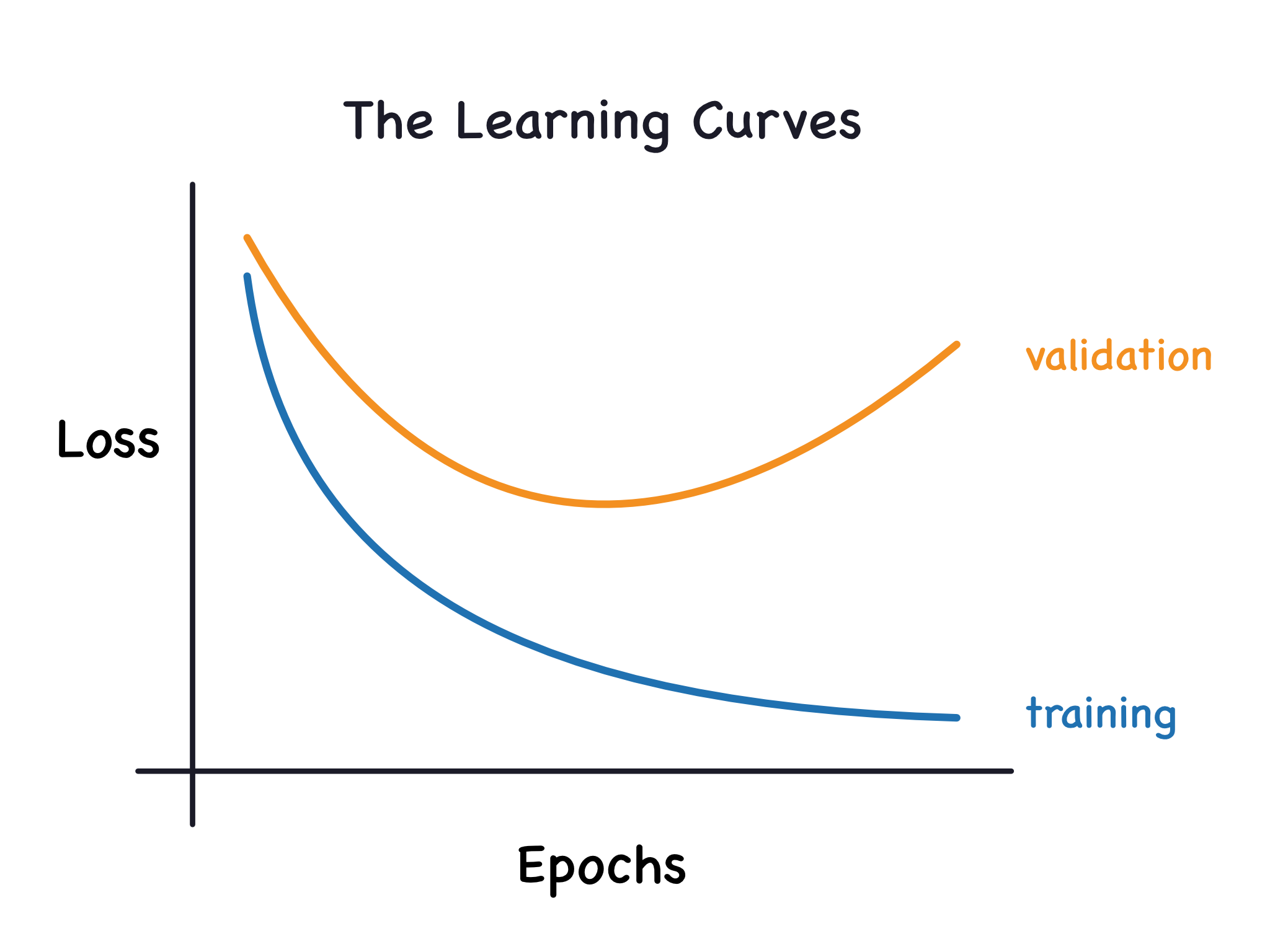
where the model starts learning too much noise from data and not just the underlying signal that needs to be modeled. This causes the accuracy on the training set to continually improve, naturally, but have it lose its ability to generalize, indicating an increase in validation loss (or a decrease in validation accuracy).

In the case of underfitting, it’s a little bit harder to tell. Generally, the learning curve will look relatively similar to an ideal learning curve where both training and validation curves are close together, but both accuracies will be low, indicating poor learning (stressing that the closeness of the two curves doesn’t really imply a reassuring generalizability, but rather that it performs similarly poorly on a training and validation set).

All in all, learning curves are an incredibly important diagnostic tool for the health of your model. Both cross-validation and learning curves aid the machine learning engineer in diagnosing and limiting bias and variance, so that we can better arrive at that optimal estimator.

References

Henry (https://math.stackexchange.com/users/6460/henry), difference between bias vs variance, URL (version: 2020-05-10): https://math.stackexchange.com/q/3667818

Van Dusen, Ben & Nissen, Jayson. (2022). How statistical model development can obscure inequities in STEM student outcomes. Journal of Women and Minorities in Science and Engineering. 28. 10.1615/JWomenMinorScienEng.2022036220.