The misconceptions of the imbalanced dataset
A common pitfall a beginner machine learning engineer can find themselves in is putting faith in the metric “accuracy”. In classification tasks, accuracy is defined as:
\[\frac{P_T + N_T}{P + N}\]Where \(P_T\) and \(N_T\) represent the true and false positive results respectively made by a predictor, whereas \(P\) and \(N\) represent the actual number of positive and negative cases in something like a test dataset. It’s quite easy to compute when programming as long as your == operator is element-wise, and computing it between \(y\) and \(\hat y\): the true and predicted \(y\) values. This will create an array of booleans whose average is the accuracy.
Accuracy as a metric is rife throughout machine learning libraries like Tensorflow, where validation accuracy is a common early stopping criterion for training. Accuracy is a fine metric, but it can lead you astray if you use it too liberally.
Where accuracy goes wrong
Suppose a bank wants to create a classifier than determines whether bank transcations are fraudulent (1) or not (0). Suppose someone is tasked with creating this model, and trains a support vector machine, or maybe a basic decision tree for interpretability. Suppose that when they train the model, they rely on validation accuracy as a stopping criterion.
Suppose they start training, and all of a sudden the model is trained quickly and in a few epochs, with validation accuracy well over 90%. This should be an expected result if you looked at the target distribution, and you would probably not consider this model well-equipped to handle its use case if you were willing to allow it to be better at catching fraud at the cost of sometimes flagging fraud where there is none. For the model used, I can create my own predictor that will likely do just as good a job in one line of code: def predictor(x): return 0
If the engineer were to look at his data, if the data is representative of a typical bank transactions dataset, fraudulent transactions would be horribly under-represented. This is an example of an imbalanced dataset, An imbalanced dataset is any dataset where the class distribution is not uniform for all classes. A balanced dataset is below, with arbitary classes \(A\) and \(B\).
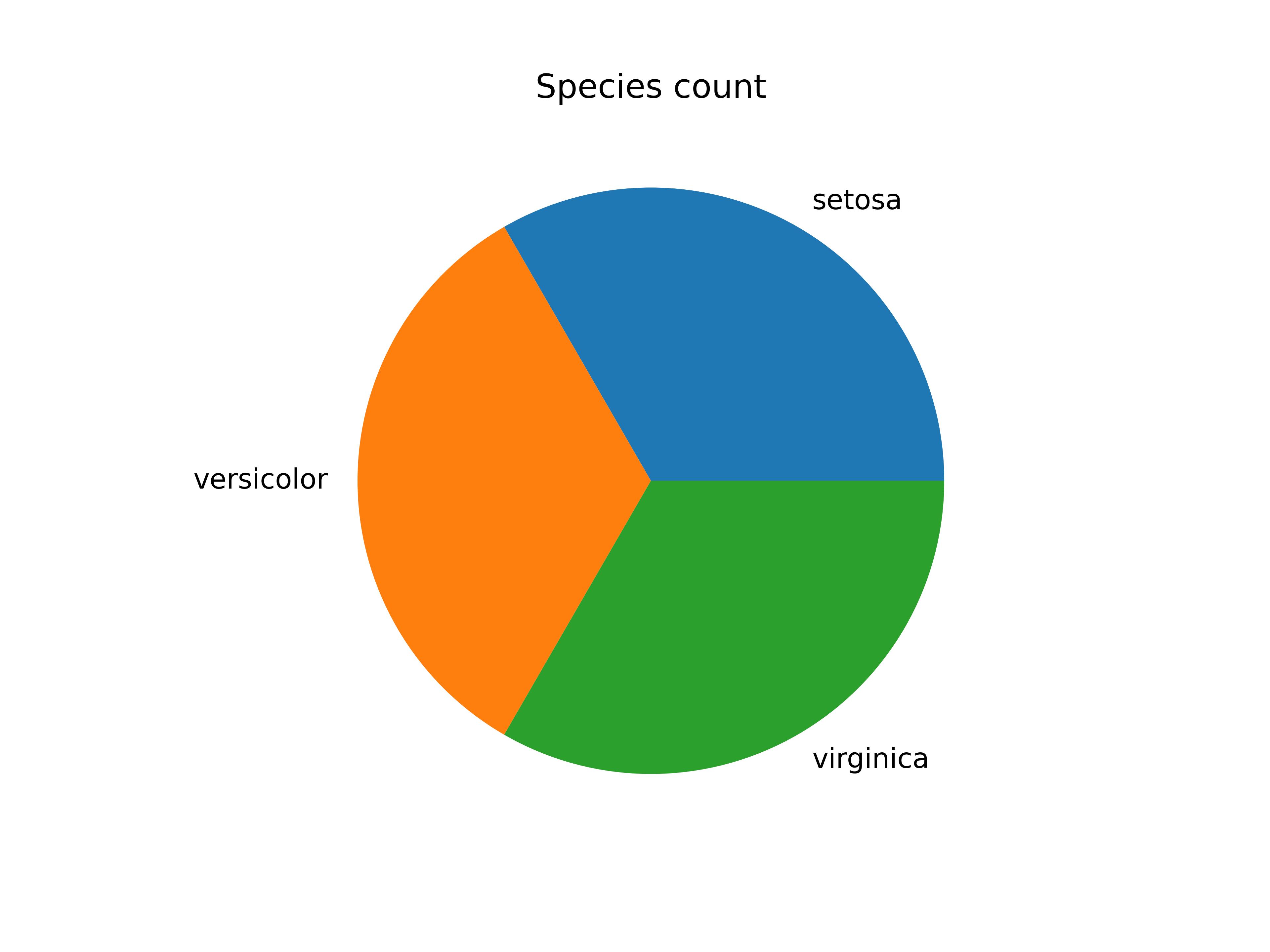
Whereas an imbalanced dataset is any deviation from this parity, such as if I reduced the prevalence of some classes at random like below:
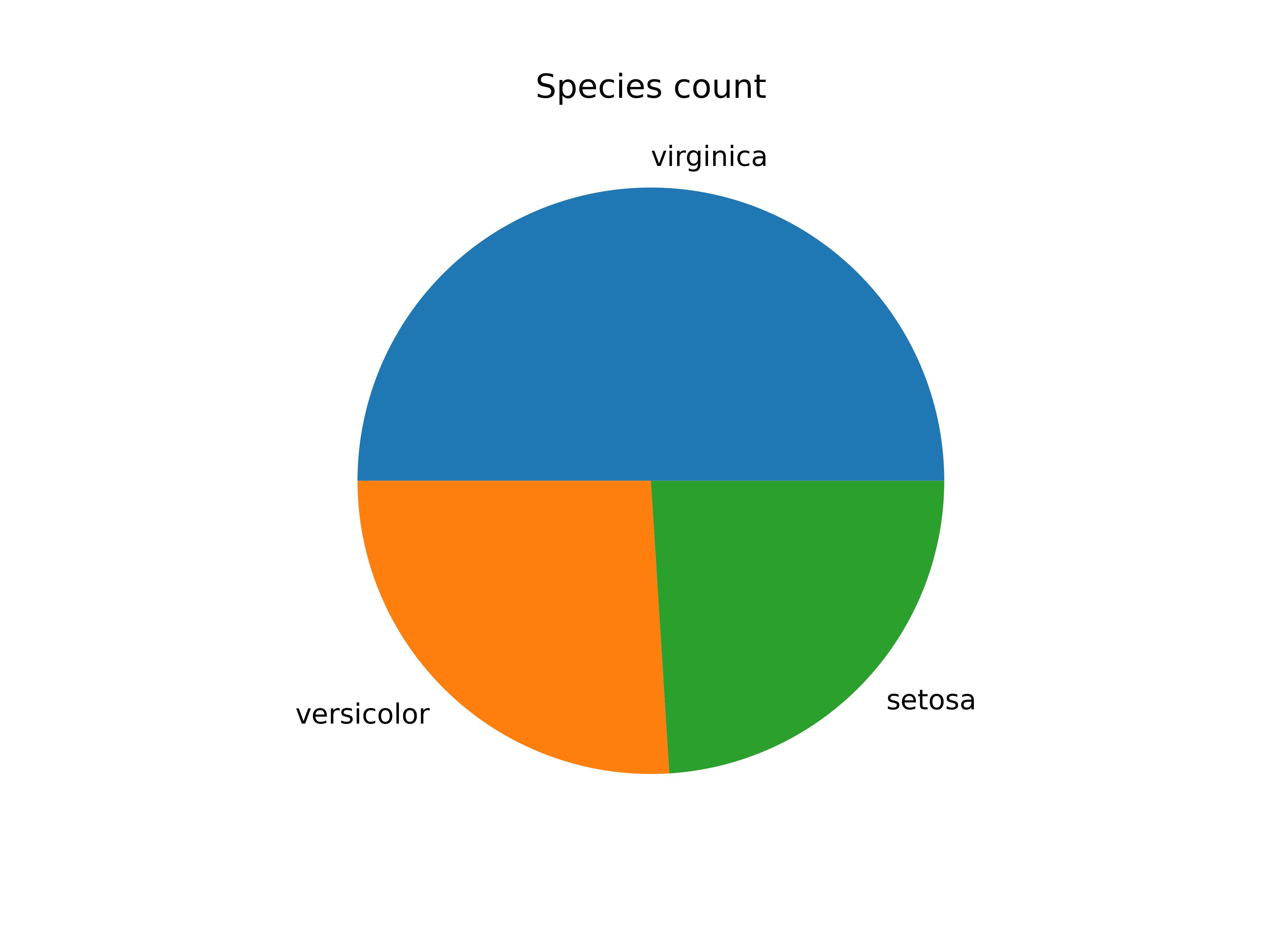
Histograms are by far the more standard way of displaying this, but I like pie charts. The first image is fairly straight-forward to train, but unrealistic – you’ll probably find it is seldom the case that this parity will occur naturally.
Imbalanced datasets are a messy subject. Once aspiring machine learning engineers learn about imbalanced datasets, they tend to invariably assume it is a problem that needs to be fixed. One of the main reasons for writing this article is as a PSA for machine learning engineers.
Ladies and gents: the issue isn’t that there is class imbalance. The issue is that you actually aren’t priotizing accuracy and don’t realize, and instead are dealing with a cost-sensitive learning problem. That is to say that the misclassification costs are imbalanced, just like your dataset.
Why models favor the majority class
Lack of complexity
Your model is probably ignoring the minority class because it is lacking the complexity to capture the patterns of the under-represented class and/or also is typically incentivized to favor the majority class when you pick a loss function and expect it to do things other than minimize with equal misclassification cost.
To explain my first part, suppose I’m using a support vector machine to separate class \(A\) and \(B\) with a hyperplane on the feature space. If I have a huge dearth of datapoints for class \(B\), it’s incredibly difficult to find a reliable hyperplane orientation to separate the classes. With more datapoints, the data cloud for \(B\) will ideally become more visible, which will allow the model to have less trouble fitting its hyperplane.
Additionally, if I worked with another primitive model like a decision tree, which recursively partitions the feature space based on chosen feature values, too little data might cause the tree to not have enough information to distinguish the minority class \(B\) from \(A\).
This can be remedied to some extent with a more complex model like a neural network, thanks to its ability to fit non-linear decision boundaries quite well. Even still though, it might not be enough.
Loss function assumes equal misclassification loss
Cross-entropy is arguably the most widely used loss function for classification tasks, and is defined for two probability distributions \(P\) and \(Q\) as:
\[H(P,Q) = - \sum_{i=1}^N p(x_i) \log{(q(x_i))}\]where \(p(x_i)\) is interpreted as the true distribution and \(q(x_i)\) as the predicted distribution. In this case, \(x\) does not refer to feature vectors, but output vectors – a vector of classes. Remember that loss functions deal with comparing output vectors.
This is why I kind of like writing it in terms of the dot product. This is the cross-entropy loss for datapoint \((x_i,y_i)\).
\[L = -\mathbf{y} \cdot \log{(\mathbf{\hat y})}\]where \(L\) now represents cross-entropy as a loss function, \(\mathbf{y}\) as the vector of values consisting of \(p(x_i)\) and \(\mathbf{\hat y}\) as the vector of values consisting of \(q(x_i)\).
The computation of which, looks like this for binary cross-entropy:
\[L = - \sum_{i=1}^2 y_i \log{(\hat y_i)}\]Subject to the fact that for specifically binary classification \(y_2 = (1-y_1)\). Cross-entropy is super nice for classification because it’s convex (which is obviously ideal for a loss function) and well-suited to backpropagation. The logarithm in its equation is also particularly handy, punishing incorrect classifications (due to its behavior \(x \to 0\)) by blowing up if the probability of the correct class is low. It also handles multiclass beautifully by simply adding more terms to the sum.
For our example here, suppose the real data has class \(A\) appear 90% of the time and class \(B\) appears 10% of the time, and suppose for the sake of the example our predictor is perfectly calibrated and wants to predict class \(A\) 90% of the time and class \(B\) 10% of the time as is the case in the real data (a calibrated predictor means its predicted probabilities match the true probabilities, implying that if a class appears 90% of the time in a dataset its average prediction probability is 90%) . That leaves our loss function as follows, if we are solving for 100 datapoints. I’ll start with the total loss over all the datapoints
\[L = \frac{1}{100} \sum_{i=1}^{100} -\mathbf{y}_i \cdot \log{(\mathbf{\hat y}_i)}\]where each vector is two-dimensional. This can be expanded as:
\[L = - \frac{1}{100} \sum_{i=1}^{100} \sum_{j=1}^2 y_{i,j} \log{(\hat y_{i,j})}\]And to calculate..
\[L = - \frac{1}{100} \left(90(1 \times \log{(0.90)} + 0 \times \log{(0.1)}) + 10(0 \times \log{(0.90)} + 1 \times \log{(0.1)})\right)\] \[L = 20.81...\]Keep in mind I’m slightly taking liberties here for the sake of explanation, assuming that each time it predicts the positive and negative class with the same probability due to it being calibrated – on average this will be the case but it is unlikely to all be exact. If our predictor is no longer calibrated and on-average predicts class \(A\) 99% of the time and class \(B\) 1% of the time regardless of how often either class appears in the training data..
\[L = - \frac{1}{100} \left(99(1 \times \log{(0.99)} + 0 \times \log{(0.01)}) + 1(0 \times \log{(0.99)} + 1 \times \log{(0.01)})\right)\] \[L = 4.56...\]Which is a drastically smaller loss. In order to minimize loss, therefore, models are tempted during learning to apply healthy probabilities to majority classes regardless of its actual prevalence as this lowers loss. This, however, is not necessarily a bad thing. In fact, this is actually what you want if your goal is accuracy, as this is the best way to do maximize it.
The reality of imbalanced datasets
The above behavior is only an issue if the cost of misclassifying one class should be higher than the cost of misclassifying another (this problem often appears in the medical field where misclassifying a false negative for a malignant tumor is far worse than misclassifying a false positive for a malignant tumor). That is to say that an accurate prediction isn’t the most important thing. If your data is representative and you are only interested in accurate prediction, this behavior is optimal, as it has optimized your accuracy. You’re done.
So, when we’re interested in good performance on a minority class to the point where we’re willing to eschew a bit of overall accuracy, we’ll need to add some way to favor minimizing the loss by better predicting minority classes.
Let’s briefly return to the example from before. The calculation I was effectively doing per datapoint is commonly written as:
\[L = -(y \log{(p)} + (1-y)\log{(1-p)})\]Suppose we tack on a constant to the first term:
\[L = -(\alpha y \log{(p)} + (1-y)\log{(1-p)})\]As this is once again an example for binary cross-entropy, I should note that the first term traditionally relates to what is called positive error, as it refers to the error made by the classifier when it misclassifies a positive instance (a label of \(1\)) as negative (a label of \(0\)), and vice versa for the second term – the negative error. If \(0 < \alpha < 1\), we buffer the penalty of positive error, incentivizing precision at all costs and causing even greater minority exclusion. If \(\alpha > 1\), we exacerbate positive error in favor of negative error, incentivizing better recall by reducing false negatives. When considering this, remind yourself that a term closer to \(0\) in the logarithm for the non-zero term in the sum is a misclassification. This is one way to combat misclassification cost, known as weighted cross-entropy. For multiple classes, you turn your scalar \(y\) that can be \(0\) or \(1\) into a one-hot vector where the correct class gets a \(1\) and the rest get a zero, and your probability is now a vector of probabilities (softmaxxed from your model) corresponding to the probability of each label.
This is a fairly conventional way of introducing weighted cross-entropy, but I could’ve just as easily gave both terms their own constants. The point is that when the “wrong class” is classified (the term with a value of \(p\) that is not the highest of all the other terms), and that term corresponding to its classification is the only term left standing, the scalar you give it will modulate the loss you accrue; larger weights exacerbating misclassifying and lower weights being “more forgiving”. Weighted cross-entropy, then, for an arbitrary number of classes \(m\) can be written as for datapoint \((x_i,y_i)\):
\[L = -\mathbf{y^w} \cdot \log{(\mathbf{\hat y})}\]where I’ve denoted \(\mathbf{y^w}\) as the Hadamard product of the original ground truth \(\mathbf{y_i}\) and a weights vector \(\mathbf{w}\) such that \(\mathbf{y^w} = \mathbf{y} \odot \mathbf{w}\). This can be written as for \(m\) classes:
\[L = - \sum_{i=1}^m y^w_i \log{(\hat y_i)}\]So that for a minibatch of \(100\) datapoints, our loss would be:
\[L = - \frac{1}{100} \sum_{i=1}^{100} \sum_{j=1}^m y^w_{i,j} \log{(\hat y_{i,j})}\]Reminding ourselves that \(\mathbf{\hat y}\) is the output of the model, a vector of probabilities for each class, no different than simply \(p\) from the binary case. I could’ve easily called it \(\mathbf{p}\) but model outputs are traditionally written as \(\hat y\) and I like to keep to convention. Speaking of convention, I really wish \(i\) and \(j\) weren’t common letters used for indices because I hate how the comma and the \(j\) get all smushed with something like \(x_{i,j}\). Boo!
Another way to help minority class prediction would be to adjust decision boundaries after the fact to allow minority classes more leniency to be predicted.