ChatGPT has blown up the world of ML and seems to have transcended all other machine learning innovations since I’ve entered the field, seemingly heralding a new epoch (no AI pun intended) of artificial intelligence. Ever since it came out in November I’ve been using it constantly for things work-related and non-work-related. I’m going to attempt to give a detailed look into how ChatGPT works. This will be relatively heavy on concepts so that it can be lighter on substance to where it’s not a 90-minute read. Consider this a read for someone passionate in the field and knows a few basic concepts already regarding NLP.

ChatGPT is an artificially intelligent chatbot developed by OpenAI that deployed last November. It’s built on top of GPT-3, which is part of what I like to consider the pantheon of NLP large language models, particularly notorious for its ability to summarize or generate text. GPT stands for Generative Pre-Trained Transformer.

This article is designed to be slightly heavier on text-generative transformers than on how ChatGPT was specifically trained, although I’ll be touching on it. The latter was summed up in HuggingFace’s blogpost better than I ever could. Also, I don’t get in to some stuff typical to reinforcement learning like policy gradient methods, so if you’re unfamiliar with that kind of stuff it may be worth doing a bit of reading into it. There’s a lot of great resources out there, and you can always try asking ChatGPT! Just make sure you validate it using a human source :-).

Transformers

A transformer is a complex type of neural network architecture that really has no peer in natural language processing. It’s also relatively new, debuting in a paper titled “Attention is All You Need” by Vaswani et al in 2017. It piggybacks off of sequence-to-sequence models (Seq2Seq) that takes a sequence as input and takes a sequence as outputs. Before their invention, the usage of recurrent neural networks (RNNs) were the standard. Transformers immediately seemed to eclipse RNN’s in usage due to their improved capacity to capture long-range dependencies in sequences, ability to process tokens in parallel (as opposed to sequentially, which additionally suffered from the risk of vanishing gradients) and are far more interpretable with self-attention. A transformer is shown below from the original paper:

which for me, when I first saw it, was absolutely befuddling. My hope is that after reading this article, if you go back to this graphic it’ll make a bit more sense. Let’s dive right and start dealing with the attention units. I will be describing a an autoregressive encoder-decoder transformer to generate text. I will do so by framing it in an explanation of encoders and decoders, but I want to preface this by saying: the two of them are very similar, and can be thought of as slight variations of a generic transformer block; something with multiheaded attention and an MLP.

Self-attention and the encoder

Transformers are composed of things called scaled dot-product attention units. These attention units embed the input document by each token’s weighted relevance to other tokens in the sentence.

For each attention unit, the model learns weights matrices \(W_Q\), called the query weights matrix, \(W_K\), the key weights matrix, and \(W_V\), the value weights matrix.

Suppose we have a document \(d\) with \(n\) tokens that I will describe in terms of their embeddings: \(d = (u_1, u_2, ..., u_n)\), which we can assume are produced using a pre-trained word vector space like GloVe or something. For each token, we produce a query, key and value vector by multiplying the token’s embedding with each of their associated weights matrices.

Therefore, for a position \(i\), corresponding to a token \(t_i\), we have a query vector \(q_i = u_i W_Q\), a key vector \(k_i = u_i W_K\) and a value vector \(v_i = u_i W_V\). Then, for each position \(i\), we get an attention weight between positions \(i\) and \(j\) by taking the dot product of \(q_i\) with \(k_j\):

\[\alpha_{i,j} = \frac{q_i^T k_j}{\sqrt{n}}\]

which can be thought of as the relevance of token \(i\) on token \(j\). These attention weight are computed for all \(n\) tokens, so that for token \(i\) you have a vector of attention weights \((\alpha_{i,1}, \alpha_{i,2}, ... , \alpha_{i,n})\). This inclues an attention weight for itself, \(a_{i,i}\). The vector is softmaxxed so that all the scalars add up to unity, and to denote that I will rewrite the attention weights as \((a_{i,1}, a_{i,2}, ... , a_{i,n})\). This vector then acts as weight for the weighted sum of value vectors for each position, creating a vector of attention units.

\[\text{Attention}_i = \sum_{j=1}^n a_{i,j} v_{j, i}\]

Packing each \(\text{Attention}_i\) into a matrix is considered the formal calculation for an attention head. Indeed, it is common to combine all the query vectors into one query matrix \(Q\), all key vectors into one key matrix \(K\), and all value vectors into one value matrix \(V\) so that you can express the above equation as:

\[\text{Attention} = \text{softmax} \left(\frac{QK^T}{\sqrt{n}}\right) V\]

Where you might define \(\text{softmax} \left(\frac{QK^T}{\sqrt{n}}\right)\) as an attention weights matrix \(A\).

By doing this for all tokens, you’ve self-attended your document \(d\). Notice that through all these vectorized operations we’ve managed to enable full-range context dependency on all of our tokens, which RNN’s aren’t able to do. In addition, this setup allows for asymmetry between tokens \(i\) and \(j\). As \(\alpha_{i,j} \ne \alpha_{j,i}\), this means that the influence of token \(i\) on \(j\) can be large while the influence of token \(j\) on \(i\) can be mild and vice versa.

One set of weights matrices each is referred to as an attention head, and each attention layer will have multiple heads, as you can see from the “multi-head attention” stuff in the above image. The reason why you want to use multiple heads is similar to why you want to use multiple hidden layers in a neural net, in that it allows more insights to be picked up by combining the “ideas” of all the heads.

The final multi-headed attention’s output is a concatenation of all of the attention vectors multiplied by a final weights matrix \(W_O\):

\[\text{MultiheadAttention(Q,K,V)} = \text{Concat}(\text{Attention}_i)W_O\]

which is fed to a feed-forward neural network as essentially an “enhanced” version of a word embedding, holding more contextual information through self attention, sometimes called a thought vector.

This was a lot, so let me summarize:

The traditional function of an encoder is for each document it receives is to endow each token \(u_i\) with key, query and value vectors. - Each token attends to every token in the document, including itself, performing a normalized dot product with its own query vector with every key vector from the tokens in the document, creating a vector of attention weights \((a_{i,1}, a_{i,2}, ..., a_{i,n})\).
Each token’s attention weights are then dotted with its value vector to compute its vector of attention units \(\text{Attention}_i\)
Each vector of attention units for each token are combined as the final output for an attention head: a matrix corresponding to all of the attention unit vectors for each token thrown in a matrix.

It’s usually then passed to an \(\text{Add&Norm}\) layer which adds the input used to generate the output with that latter output. That sounds confusing, but for example the first \(\text{Add&Norm}\) layer adds the input embeddings with the result of the first multi-head attention layer, and the second layer adds the output of the feed-forward layer to the output of the multiheaded attention layer (which serves as the \(\text{Add&Norm}\) input as it’s used as output for the feed-forward). \(\text{Add&Norm}\) layers help to reduce the risk of vanishing gradients.

This is known as an encoder. There usually are a number of these in popular transformers. The first encoder takes word embeddings as input, while the subsequent encoders take encodings.

I’m going to skip positional encoding other than to say it provides a way to capture the order of an input sequence, which is good because otherwise it couldn’t distinguish between two tokens that have the same value vector but appear at different positions in the input sequence.

I also recommend you give this article a look if you want a visual explanation. It’s lovely.

Decoders

The decoder is responsible for actually producing the output. For text generation, it takes as input the previously generated output tokens in the output, and the output of the encoding layers. If no tokens have been generated so far it starts with a start-of-sequence token \(\text{SOS}\).

Firstly, self-attention is applied to the output tokens. In order to ensure the decoder doesn’t “cheat” and use current or future output tokens in its autoregressive generation, it uses a attention layer that masks tokens ahead of token \(t\) before the softmax stage. Then, the encoded input and previously generated tokens are all used as input for another multi-head attention layer, which allows it to focus on relevant parts of the input sequence to generate the next token. Another way of saying this is that the decoder attends to the encoded input as well as the previously generated tokens.

This net encoding of the encoded input with the previously generated tokens is finally used as input for a feed-forward neural network, which produces a softmaxxed probability distribution of likely next tokens, and this process iterates until you hit a max token length or an end-of-sequence token \(\text{EOS}\). A transformer like GPT was trained by merely feeding it sequences: the text input serves alone as training data as you compare the next token to the real next token in the sequence.

Yes, that’s pretty much the gist of it. It’s complicated, but if you were to take anything away, it would be this:

Transformers leverage context between tokens in each sequence, not just a token’s embedding, all without a dependency range limit.
Text-generation transformers leverage context between tokens in an input sequence to tokens in their output sequence, as well as the output sequence with itself.

This is the basic transformer architecture for text generation, and most of the famous transformer architectures you hear about (like BERT or GPT) are all slightly different. BERT for one, is bidirectional (hence the ‘B’) while GPT is unidirectional (it can only see current or preceding tokens). BERT uses masked attention layers during its pre-training to try and leverage context to try and guess the masked tokens, while GPT is more in line with what I’ve explained here. They’re all transformers but may have been pre-trained differently and this allows them to have certain strengths or weaknesses over others (such as GPT’s pre-training using next token prediction making it a bit better suited to text generation, BERT’s masked token prediction and bidirectional encoding making it a bit better at virtually everything that isn’t text-to-text generation, etc).

Semantic temperature

ChatGPT word-for-word selects from a probability distribution of every token in its massive corpus. If the highest probability tokens are always selected, this tends to make for unrealistic messages.

Recall that the final layer of a transformer is a softmax scaled on output vector \(\vec z\). A vector component \(z_i\) would then be transformed like:

\[\sigma(z_i) = \frac{e^{z_i}}{\sum_{j=1}^{N} e^{z_i}}\]

but introduce an additional parameter \(\tau\) like so:

\[\sigma(z_i, \tau) = \frac{e^{z_i/\tau}}{\sum_{j=1}^{N} e^{z_i/\tau}}\]

where \(\tau\) is called the semantic temperature. In order to better understand how this affects the output logits, consider some edge cases.

\(\tau \to 1\). reverts to the original softmax.
\(\tau \to 0\) reduces to argmax. See EDZ’s answer on stack exchange where \(1/\tau \to 0\) is equivalent to \(c \to \infty\) in the user’s example.

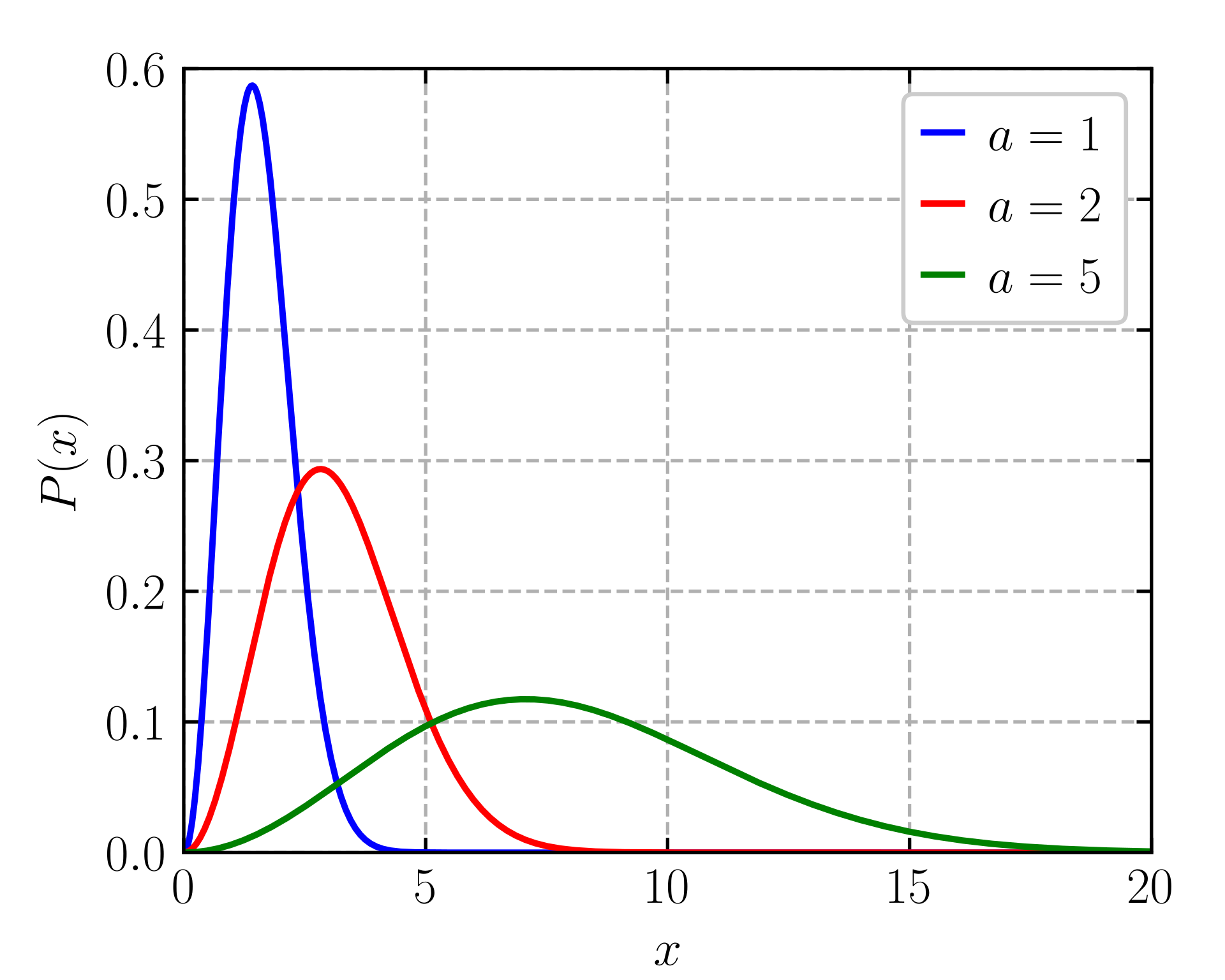
Generally speaking, when temperature is computed it’s usually applied to the logits \(\text{logit} \to \frac{\text{logit}}{\tau}\) before being applied to the softmax. At lower temperature \(\tau\), the resulting probability distribution over the classes becomes exponentially “sharper”, exacerbating the gap between higher probability and lower probability outputs, hence why \(\tau \to 0\) tends to argmax. Larger values of \(\tau\) will blunten the probability distribution over the classes, allowing previously lesser probability tokens to have a higher chance of being generated as the smoothing is harsher for higher logits. The softmax in general is an analog to the Gibbs distribution in statistical mechanics. In the Gibbs distribution, lower temperature cause the distribution to be more pointed.

Below is a plot of the Maxwell-Boltzman distribution as temperature varies. It’s not the exact same as the Gibbs distribution or temperature-dependent softmax, but it captures the same blunting with increased temperature that I’m referring to. Note that here \(a \propto T\).

ChatGPT, by its own admission, uses a temperature-annealing process during its training, in order to encourage exploration of different next tokens early on (which will also help in preventing overfitting) and encouraged to converge to more “safe” or “accurate” outputs towards the end.

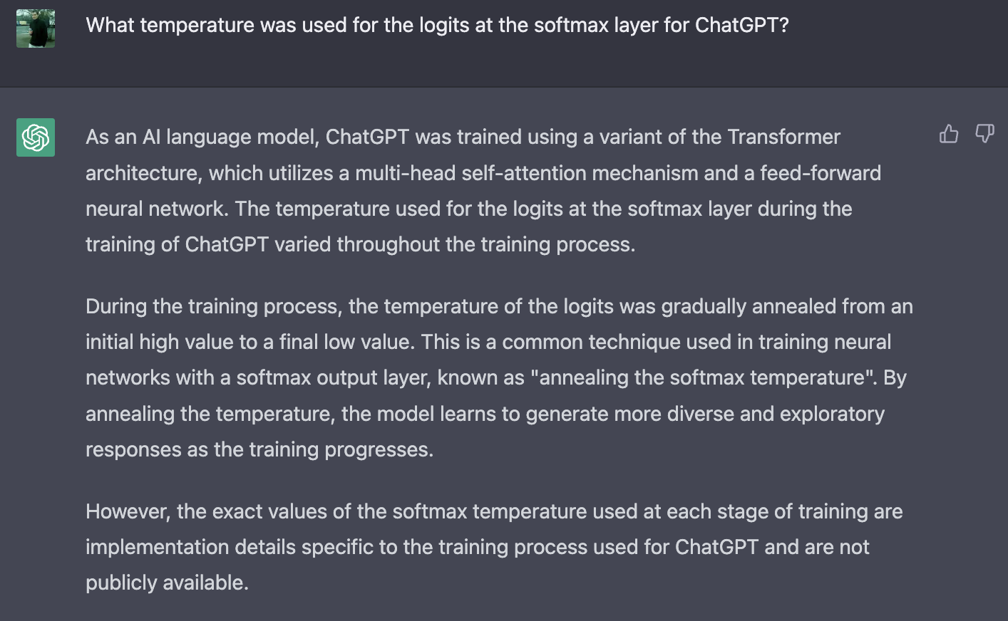
That being, said ChatGPT’s factual accuracy isn’t always perfect so this should be taken with a grain of salt.

How ChatGPT was trained

ChatGPT’s training process was far more complicated than that of a typical transformer, eschewing supervised, semi-supervised and unsupervised learning for training its primary language model in favor of a new paradigm called reinforcement learning with human feedback. I’m going to refrain from explaining reinforcement learning much at all in favor of preserving some semblance of brevity for this article.

In reinforcement learning, an actor aims to act according to a policy in order to maximize a reward. In NLP, a natural challenge was trying to define a reward that wasn’t so easy as “distance to checkpoint” or “distance from soccer ball to goal” that didn’t just cause text generation models to “cheat the system” by producing gibberish that garnered high reward scores. Attempts were made to define rewards in terms of how favorable it would be to humans such as BLEU or ROGUE, but these weren’t ultimately super satisfactory. Reinforcement learning with human feedback (RLHF) aimed to remedy this with a more clever reward metric: a language model. It’s a relatively new concept, as 2019 is the earliest paper I can find on the subject.

Reward models

A reward model is a language model (a transformer) trained to identify whether a prompt is useful to humans or not. One way I’m aware it can be done is by providing putting two language models on a prompt and ranking which one is better, generating a sort of ELO system like it’s chess. Giving a blank score to a prompt has been found to be ineffective, as human labelers tend to be less likely to see eye-to-eye on an exact score as opposed to a picking a favorite out of two, causing noisy training data.

Once the reward model is trained, we’re left with a text-generation transformer and a reward model that ideally is able to distinguish useful prompts from not-so-useful prompts.

The process

A general outline of the fine-tuning process can be visualized with a lovely visual from HuggingFace’s blogpost on RLHF, which explains this whole process in great detail:

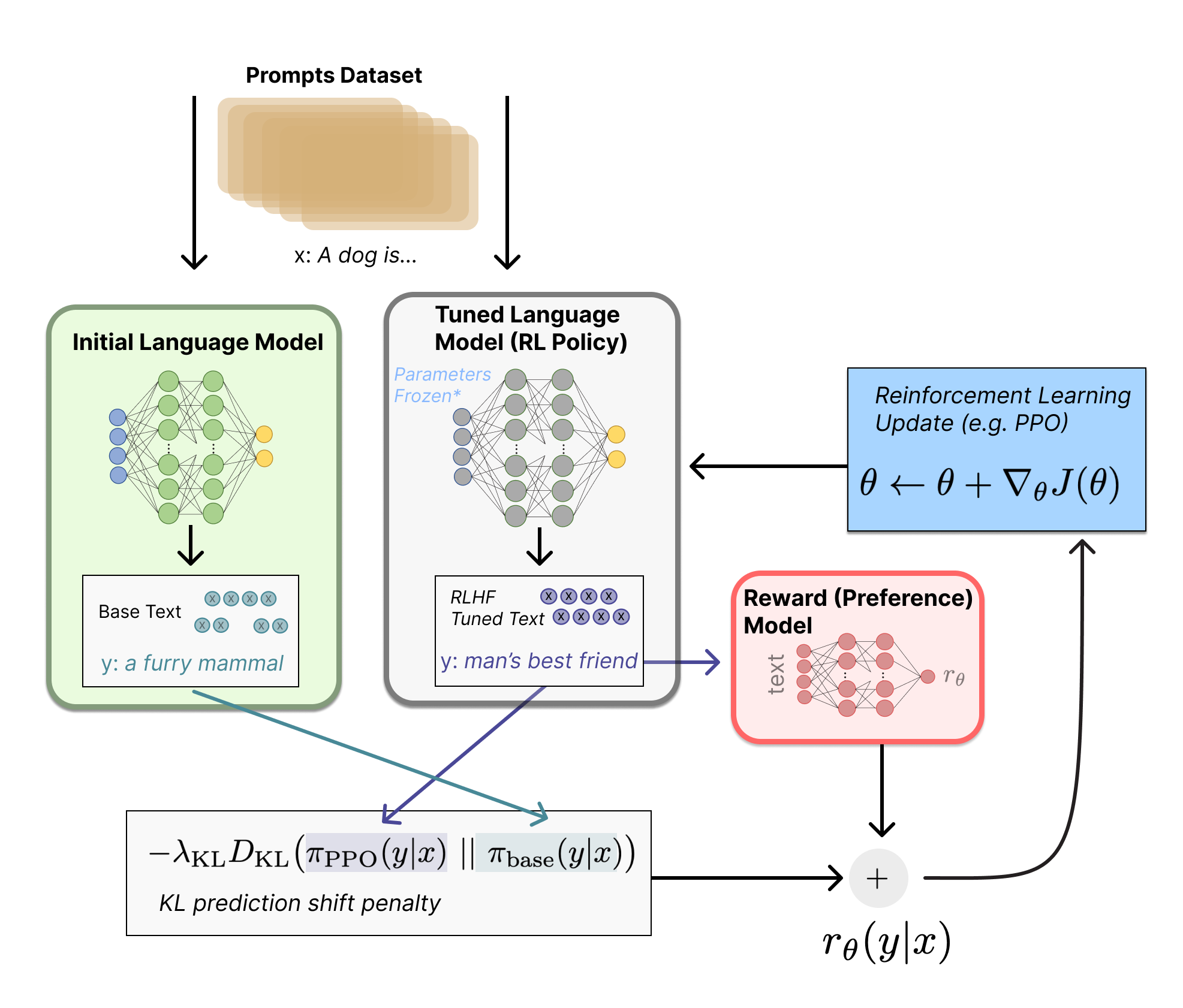
and to annotate this process:

Two LM’s are used that can generate text. All the LM’s in use tend to have billions of weights, including the reward model. One LM is used to be fine-tuned for optimal responses in this process, called the policy, and another is used as a control to help stabilize the policy’s outputs.
Both LM’s receive a prompt and generate text. The policy’s text is scored by the reward model, rendering score \(r_{\theta}\) and the initial LM and the policy’s outputs are combined to generate a Kullback-Leibler divergence score \(r_{KL}\) that is a further hedge against the policy cheating the reward model with gibberish by penalizing responses that venture too far from the initial LM’s output.
This adjusted reward score \(r = r_{\theta} - \lambda r_{KL}\) (with \(\lambda\) serving as a scalar to modify the magnitude of the KL divergence’s penalization) is fed to a policy gradient method called proximal policy optimization (PPO). PPO is a trust region optimization algorithm, which for brevity essentially aims to update the policy to maximize the reward metric without letting it verge too far from the old policy (hence “proximal”). It essentially takes a ratio of the probabilities of producing a specific output under the new policy versus the old policy, and clipping a policy update to a maximum amount if that ratio is too large. There has been discussions about updating the reward model together with the policy model, but at the time of this writing I don’t think it’s been done yet.

This process is repeated until, I assume, the prompts dataset is exhausted or some early stopping criterion is reached (such as policy updates tapering off).

Some things to note

To describe as much as possible, I talked about an encoder-decoder transformer, but not all LLM’s are based off this design. Some, like BART, are in this framework, while BERT is an encoder-only model, and LLM’s like GPT (all generations) and LlaMa are decoder-only (Bard might be too but I’ve read conflicting information on it).
Decoder-only transformers are more common for autoregressive text generation LLMs. They don’t seem to have any need for encoders because there is seemingly not much benefit to learning the latent vector representation of the input sequence when only attending to currently generated tokens.

Encoder-decoder transformers seem to work great for applications where long-range contextual understanding of the input sequence is important (encoders are great for this) and text generation is desired (decoders), like with language translation.

It may seem like no explanation as to how ChatGPT was trained seems to make its remarkable usefulness believable. My only explanation for this would be the likely exorbitant amount of training data and parameters at play here.

ChatGPT released their API recently, and with it, an option to control its temperature. It would be interesting to see how it does with more “safe” or exploratory responses.

Because of the way the reward model was trained, ChatGPT is designed to generate prompts that are useful to humans. This does not mean that it’s factually accurate, and I highly recommend not relying on ChatGPT to learn things without having enough information to know if it’s making any sense beforehand.

There are likely tons of other things that ChatGPT makes use of under the hood that OpenAI has not publically disclosed. I’m not aware of how it handles continuing conversations or correcting itself beyond a few complete guesses.

One of the limitations listed on ChatGPT’s main page in the chat window is that it has “limited knowledge of world and events after 2021”. That implies that there is limited training data that exists in 2021 or later. One of the biggest issues with serving trained models is concept drift, which is a model’s declining usefulness with time since training. I suspect ChatGPT’s advice can and will become dated in the future, and it will probably be up for a costly re-training in the near future given how widely used it is, which will present a constant financial load to provide ChatGPT as a service on the part of OpenAI. Given recent investment, however, I’m not too worried for them.

References

Wikipedia contributors. (2021, December 30). Transformer (machine learning model). In Wikipedia, The Free Encyclopedia. Retrieved 20:43, March 3, 2023, from https://en.wikipedia.org/wiki/Transformer_(machine_learning_model)

Jia, R., & Liang, P. (2017, September 15). Maximum Likelihood Decoding with RNNs: The Good, The Bad, and The Ugly. Retrieved March 3, 2023, from https://nlp.stanford.edu/blog/maximum-likelihood-decoding-with-rnns-the-good-the-bad-and-the-ugly/

Wolfram, S. (2023, February 28). What Is ChatGPT Doing (and Why Does It Work)? Retrieved March 3, 2023, from https://writings.stephenwolfram.com/2023/02/what-is-chatgpt-doing-and-why-does-it-work/

Hugging Face. (2021, October 27). RLHF: A Dataset for High Stakes, Multi-Agent RL. Retrieved January 4, 2023, from https://huggingface.co/blog/rlhf

Vaswani, Ashish; Shazeer, Noam; Parmar, Niki; Uszkoreit, Jakob; Jones, Llion; Gomez, Aidan N.; Kaiser, Lukasz; Polosukhin, Illia (2017-06-12). “Attention Is All You Need”. arXiv:1706.03762 [cs.CL].

Salamone, L. (n.d.). What is Temperature? Retrieved March 6, 2023, from https://lukesalamone.github.io/posts/what-is-temperature/