Generative models, discriminative models, and what everyone gets wrong about naive Bayes
When learning about machine learning models, especially in the context of classification (and NLP), it is usually a pretty good idea to learn simpler models and then build up to more complex ones. A fairly common order is naive Bayes and then logistic regression. Logistic regression is a good precursor to more complex stuff like neural networks, as it captures all the weights optimization stuff while still being pretty interpretable. I’ve talked a bit about logistic regression in the past briefly (see my article) but haven’t delved into it formally, and I’ve never touched on naive Bayes. You probably won’t ever use them (especially naive Bayes) if you value performance above everything, but they’re still incredibly important to learn foundationally. They’re also different “philosophically”, in that they represent two different approaches to classification; naive Bayes being a generative model, and logistic regression being a discriminative model. I’m going to talk about all of this in this article, starting with naive Bayes and the generative model. I’m also going to get into this towards the end: naive Bayes is not traditionally a linear classifier, and I explain why.
Naive Bayes and the goal of Classification
The naive Bayes model for classification in NLP is a good next thing to learn after starting with the \(n\)-gram model. The goal of any classifier \(\hat c\) is to satisfy the following:
\[\hat c = \underset{c \in C}{\text{argmax}} \ P(c|d)\]The naive Bayes classifier then applies Bayes’ rule in statistics:
\[P(x|y) = \frac{P(y|x)P(x)}{P(y)}\]such that it views a classifier’s task as
\[\hat c = \underset{c \in C}{\text{argmax}} \ \frac{P(d|c)P(c)}{P(d)}\]Since we are computing the equation above for each possible class, \(P(d)\) is a constant throughout all our calculations and can be discarded as it has no bearing on the result. Therefore we can express it as:
\[\hat c = \underset{c \in C}{\text{argmax}} \ P(d|c)P(c)\]Naive Bayes is called a generative model. \(P(d \vert c)P(c)\) can be expressed as the joint probability distribution \(P(c,d)\) due to the conditional probability density function
\[P(y|x) = \frac{P(x,y)}{P(x)}\]for \(P(x) > 0\). As such, naive Bayes actually attempts to model the joint probability \(P(c,d)\) rather than \(P(c \vert d)\) directly. Models of this form are called generative in that they learn the joint probability distribution \(P(c, d)\) and can thereby theoretically generate documents by fixing a \(c\) and sampling documents in \(P(d \vert c)\).
Noting that a document \(d\) is a vector of features (tokens) we can express our original classifier as
\[\hat c = \underset{c \in C}{\text{argmax}} \ P(w_1, w_2, w_3, \ \ldots \ , w_n \vert c) \ P(c)\]Keep in mind that we have reached this equation with no loss of generality – this is true for all classifiers. However, the whole point of naive Bayes is arriving at the above equation and applying the naive Bayes assumption: that the probabilities given the class \(c\) for \(P(w_i \vert c)\) are ‘naively’ considered independent and are therefore able to be multiplied. The naive Bayes assumption is therefore:
\[P(w_1, w_2, ..., w_n \vert c) = P(w_1 \vert c) \cdot P(w_2 \vert c) \ \cdot \ \ldots \ \cdot P(w_{n-1} \vert c) \cdot P(w_n \vert c)\]Thus our naive Bayes classifier is:
\[\hat c = c_{NB} = \underset{c \in C}{\text{argmax}} \ P(c) \ \underset{i}{\prod} P(w_i \vert c)\]where \(i\) are the word positions in the document \(w\), so basically just making sure the product is taking into account word order. The calculation is typically done in log space to avoid underflow due to a product of probabilities, so we rewrite as:
\[c_{NB} = \underset{c \in C}{\text{argmax}} \ \log{P(c)} \ \underset{i}{\sum} \log{P(w_i \vert c)}\]We’ve now turned out classifier into argmaxxing a sum of linear sum of features. Keep that in mind for later. I’m not going to get into how naive Bayes is trained, but it uses maximum likelihood estimate to calculate \(P(w_i \vert c)\).
Naive Bayes’ assumption is generally a rather poor one, but it tends to do better than one might think given its “naivety”. Since it works using maximum likelihood estimation it scales wonderfully, handling both small and large training datasets well, and excels in higher dimensional data due to training in linear time and can ignore feature dependencies irrelevant to the classification tasks (as it ignores all of them). It also does surprisingly well in NLP since for text data, even though Naive Byaes disregards dependencies between words, often just the occurences of words in a document is enough information to make decent predictions.
Logistic regression
Let’s return to the original classification model from before.
\[\hat c = \underset{c \in C}{\text{argmax}} \ P(c|d) = P(d|c)P(c)\]A logistic regression model is a discriminative one. That is to say that instead of applying Bayes’ rule, we aim to directly calculate \(P(c \vert d)\). This is actually a key distinction. While a generative model can “understand” the classes in a sense by being able to generate examples belonging to them, a discriminative model cannot. It is purely concerned with separating classes and isn’t concerned with what characterizes them. This is because generative models force themselves to model the joint probability distribution \(P(c,d)\) to inform their predictions, while discriminative is only concerned with finding \(P(c \vert d)\). If a logistic regression classifier was trained to classify horses or humans, it won’t necessarily be able to tell you that humans have five fingers – just that they don’t have hooves. A generative model meanwhile could analogously “draw” a human.
Anyway, the way logistic regression computes \(P(c \vert d)\) is completely different to naive Bayes and more inline with “conventional” machine learning. Traditionally, it seeks to solve the probability of a positive class given feature vector \(x\) denoted \(P(y = 1 \vert x)\) and the probability of a negative class \(P(y = 0 \vert x)\). It learns from a training set a vector of weights and a bias term. Each weight \(w_i\), well, weighs \(x_i\) with a scalar value whose magnitude indicates its “importance” when making a classification prediction, and its parity representing its sway towards the positive or negative class. The bias term is tacked on to the end as an intercept. Each feature \(x_i\) is weighed by \(w_i\) and summed, then offset by bias \(b\):
\[z = \sum_{i=1}^n w_i x_i + b\]The sum is definitionally a dot product so we can succinctly express this as
\[z = \mathbf{w} \cdot \mathbf{x} + b\]What we have so far is not a probability. It is not bounded between \(0\) and \(1\). Weights are real-valued and have no implicit restriction on their magnitude, so \(z\) has unrestricted range. We’ve actually just derived linear regression. To output a probability, we need to pass this output through some mapping that constricts it between \(0\) and \(1\). Sigmoids are perfect for this. Let’s wrap \(z\) up in a sigmoid:
\[\sigma(z) = \frac{1}{1+\exp{(-z)}}\]
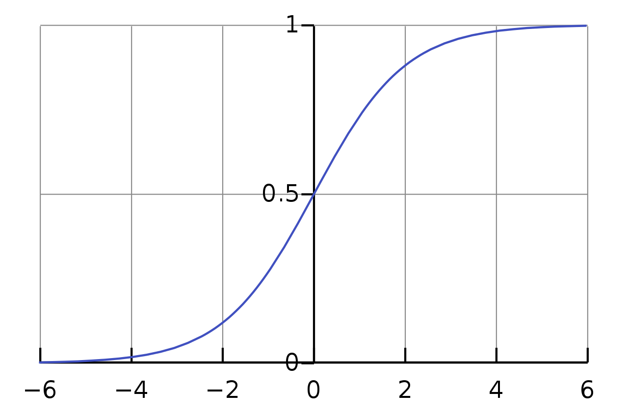
This is actually more specifically a logistic function, a specific kind of sigmoid (hence logistic regression). Sigmoids are amazingly ubiquitous in ML, and its appearance here gives a few good examples. For one, it obviously has the desired range between \(0\) and \(1\) and this prevents outliers from having an undue influence as flattening occurs near the edges. It’s also differentiable, which is always nice for models that fit using gradient descent. If we decide we want our sigmoid to model the probability that \(y = 1\), we can state:
\[P(y=1) = \sigma(\mathbf{w} \cdot \mathbf{x} + b)\]Since our only other outcome is \(y=0\), we require \(P(y=1) + P(y=0) = 1\).
Hence,
\[P(y=0) = 1 - P(y=1)\] \[= 1 - \sigma(\mathbf{w} \cdot \mathbf{x} + b)\] \[= 1 - \frac{1}{1+\exp{(-(\mathbf{w} \cdot \mathbf{x} + b))}}\] \[= \frac{\exp{(-(\mathbf{w} \cdot \mathbf{x} + b))}}{1+\exp{(-(\mathbf{w} \cdot \mathbf{x} + b))}}\]Keep in mind, logistic regression in NLP does not require a specific structure for the features – it doesn’t have to be a bag of words or word embeddings or whatever. Any property from the input can be a feature. I’ve already written an article talking about decision boundaries in logistic regression, but I want to stress that this existence of a decision boundary to make predictions is what makes this model discriminative, and its linearity is what makes it a linear classifier – that and the fact that we use a weighted (but linear) sum of features to make a prediction. Naive Bayes does this too, remember?
\[c_{NB} = \underset{c \in C}{\text{argmax}} \ \log{P(c)} \ \underset{i}{\sum} \log{P(w_i \vert c)}\]However, the topic of whether naive Bayes is a linear classifier or not is actually a bit complicated. What I’ve written above is after some assumptions, simplifications, and modifications to reduce underflow. Let’s look at this again.
An aside: a common misconception about naive Bayes as a linear classifier
If you Google whether Naive Bayes is a linear classifier, lots of stuff you’ll read will say that it is, yet at the same time looking at images of naive Bayes will show non-linear decision boundaries. What gives? Hopefully this will clear things up.
Formally speaking, a linear classifier is a model that makes a classification decision using a linear combination of its features and some scalars:
\[y = f \left(\sum_j w_j x_j \right)\]where \(f\) is some threshold function that we want to scale things from \(0\) to \(1\) for a probability and help us to establish a decision boundary. Recall that for logistic regression we literally derived
\[P(y=1) = \sigma(\mathbf{w} \cdot \mathbf{x} + b)\]Let’s start with Bayes’ rule:
\[P(c \vert d) = \frac{P(d|c)P(c)}{P(d)}\]Now applying the law of total probability (which we can because we have distinct events of \(y=1\) or \(y=0\)) to \(P(c)\) we can rewrite this as
\[P(d) = P(x_i \vert c = 1)P(c = 1) + P(x_i \vert c = 0) P(c=0)\]Denoting \(d\) as \(x_i\) but implying \(d = \{x_i\}_{i=1}^n\). Hence we have
\[P(c = 1\vert d) = \frac{P(d|c=1)P(c=1)}{P(x_i \vert c = 1)P(c = 1) + P(x_i \vert c = 0) P(c=0)}\] \[= \frac{1}{1+\frac{P(x_i \vert c = 0) P(c=0)}{P(x_i \vert c = 1)P(c = 1)}}\] \[= \frac{1}{1+\exp{\left(-\log{\frac{P(x_i \vert c = 1) P(c=1)}{P(x_i \vert c = 0)P(c = 0)}}\right)}}\] \[= \sigma \left( \sum_i \log \frac{P(x_i \mid c = 1)}{P(x_i \mid c = 0)} + \log \frac{P(c = 1)}{P(c = 0)} \right)\]This is decidedly not of the form \(\sigma(\mathbf{w} \cdot \mathbf{x} + b)\). As such, naive Bayes is not by default a linear classifier. So where does this misconception come from? The answer, as aptly answered here, is that it can be if the likelihood factors \(p(x_i \vert c)\) are sampled from exponential families.
Exponentional families form the group of common distributions you’ve heard of: normal, exponential, Bernoulli, Poisson – all exponential family distributions. If \(P(x_i \vert c)\) samples from a exponential family distribution, it can be uniquely expressed in the following way:
\[P(x_i \mid c) = h_i(x_i)\exp\left(u_{ic}^\top \phi_i(x_i) - A_i(u_{ic})\right),\]where \(h\), \(\phi\) and \(A\) are known functions. If we make the substitutions
\[w_i = u_{i1} - u_{i0}, \\ b = \log \frac{P(c = 1)}{P(c = 0)} - \sum_i \left( A_i(u_{i1}) - A_i(u_{i0}) \right)\]we can therefore restate this as
\[P(c = 1 \mid x) = \sigma\left( \sum_i w_i^\top \phi_i(x_i) + b \right)\]as shown by Stats SE user Lucas in the question I linked. As long as the sufficient statistic \(\phi_i (x_i)\) is a linear function of the features \(x_i\), this is still a linear combination of input features and therefore a linear classifier. In fact, the sufficient statistic \(\phi(x)\) for naive Bayes classifiers depends on the specific type of naive Bayes classifier used, but it always amounts to some scalar \(\gamma_i\) applied to \(x_i\). So we can actually rewrite our weights \(\hat w_i^\top = w_i^\top \gamma_i\) so our overall conditional probability is
\[P(c = 1 \mid x) = \sigma\left( \sum_i \hat w_i^\top x_i + b \right)\]So, yes, naive Bayes can be a linear classifier, but only if \(p(x_i \vert c)\) is sampled from an exponential family distribution. Otherwise it is non-linear. The cool thing about this though is that I managed to make a naive Bayes classifier and logistic regression have the same functional form given a few assumptions. This is no mistake, and it’s why the two are considered a generative-discriminative pair. You can think of the two as two sides of the same coin – quite literally (given the previous assumptions) the same model, where naive Bayes fits the probability model \(\sigma\left( \sum_i \hat w_i^\top x_i + b \right)\) to optimize the joint probability distribution \(P(c,d)\) while logistic regression fits the same \(\sigma\left( \sum_i w_i^\top \phi_i(x_i) + b \right)\) model to optimize the conditional probability \(P(c = 1 \mid x)\).
References
Lucas (https://stats.stackexchange.com/users/7733/lucas), How is Naive Bayes a Linear Classifier?, URL (version: 2015-03-18): https://stats.stackexchange.com/q/142258
Jurafsky, D., & Martin, J. H. (2019). Naive Bayes, Text Classification and Sentiment. In Speech and Language Processing (3rd ed., Chapter 4). Prentice Hall.